Code
library(tidyverse)
qualifying <- read_csv("archive/qualifying.csv")
races <- read_csv("archive/races.csv")
results <- read_csv("archive/results.csv")It’s been a while since I made my ggplot tutorials! I made those over 4 years ago, and kind of forgot how to do anything with data. However, I recently started watching Formula One, which just so happens to be a sport built off of data and analysis. So, naturally I had to relearn R and data wrangling. This whole endeavor involved a lot of Google-ing. Like, I spent an embarrassing amount of time on Stack Overflow and Reddit (both of which are great resources on the off chance that you’ve entirely forgotten the R language!).
It took me a really long time to find a dataset! There was an R package f1dataR but it hadn’t been updated since the end of the 2024 season, but I wanted the 2025 season. I eventually found this dataset on Kaggle, which had more recent races.
CSV files—short for Comma-Separated Values—are a plain text file that stores data in a table format. Basically, all the columns and rows are separated by commas, as seen below:
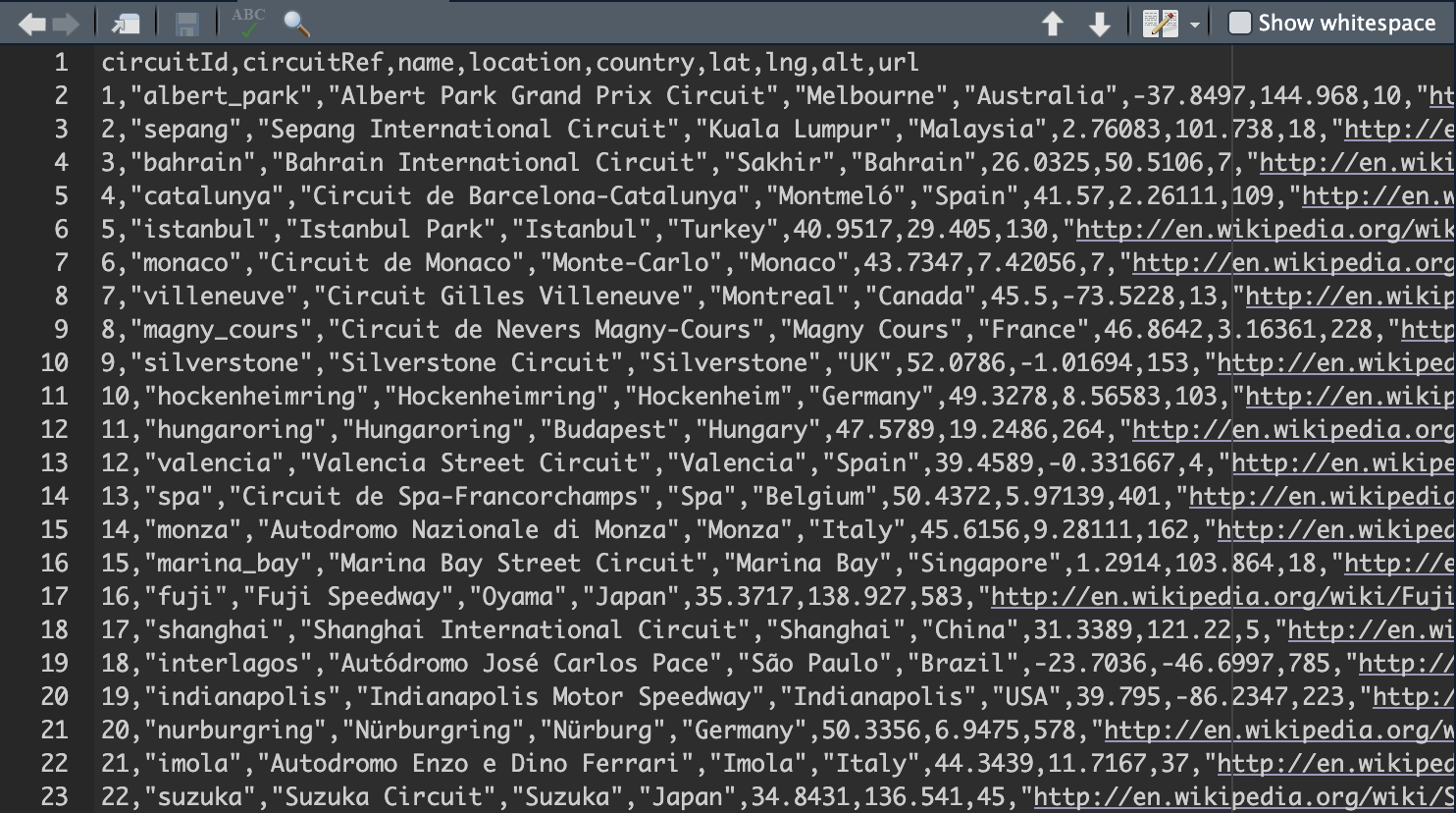
which can then be formatted as a table dataset, similar to an Excel spreadsheet:
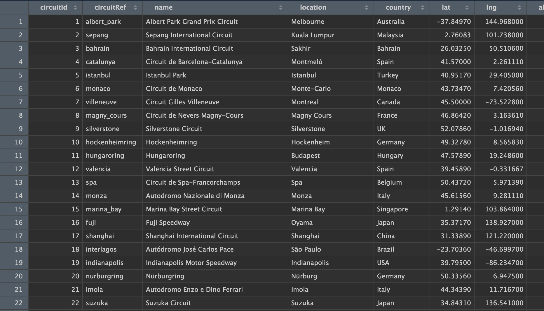
The Kaggle dataset I downloaded had a bunch of CSV files I had to get into R. After downloading, I moved the .zip file to my R project, and unzipped it, which created a folder called archive with all the raw CSV files in it. Now, I had forgotten how to use CSV files, but apparently the readr package has a function read_csv which, uh, does just that.
So the first step was to load a bunch of files into my Environment panel, which I did with read_csv. tidyverse has the readr package in it, so that is one of 2 packages I used during this adventure.
library(tidyverse)
qualifying <- read_csv("archive/qualifying.csv")
races <- read_csv("archive/races.csv")
results <- read_csv("archive/results.csv")This makes these 3 tables viewable and usable. But these tables don’t have all the columns I want.
left_join()The left_join() function comes from the dplyr package, also part of the tidyverse. It allows you to combine different datasets with matching columns. I tried combining all 3 but there were duplicate columns with different meanings, so I combined Qualifying and Races first. The dataset contains a unique ID for each race, so I was able to combine the datasets using that column.
quali <- left_join(qualifying, races, by = "raceId")

glimpse(quali)
Rows: 11,298
Columns: 26
$ qualifyId <dbl> 1, 2, 3, 4, 5, 6, 7, 8, 9, 10, 11, 12, 13, 14, 15, 16, 1…
$ raceId <dbl> 18, 18, 18, 18, 18, 18, 18, 18, 18, 18, 18, 18, 18, 18, …
$ driverId <dbl> 1, 9, 5, 13, 2, 15, 3, 14, 10, 20, 22, 4, 18, 6, 17, 8, …
$ constructorId <dbl> 1, 2, 1, 6, 2, 7, 3, 9, 7, 5, 11, 4, 11, 3, 9, 6, 10, 5,…
$ number <dbl> 22, 4, 23, 2, 3, 11, 7, 9, 12, 15, 17, 5, 16, 8, 10, 1, …
$ position <dbl> 1, 2, 3, 4, 5, 6, 7, 8, 9, 10, 11, 12, 13, 14, 15, 16, 1…
$ q1 <chr> "1:26.572", "1:26.103", "1:25.664", "1:25.994", "1:25.96…
$ q2 <chr> "1:25.187", "1:25.315", "1:25.452", "1:25.691", "1:25.51…
$ q3 <chr> "1:26.714", "1:26.869", "1:27.079", "1:27.178", "1:27.23…
$ year <dbl> 2008, 2008, 2008, 2008, 2008, 2008, 2008, 2008, 2008, 20…
$ round <dbl> 1, 1, 1, 1, 1, 1, 1, 1, 1, 1, 1, 1, 1, 1, 1, 1, 1, 1, 1,…
$ circuitId <dbl> 1, 1, 1, 1, 1, 1, 1, 1, 1, 1, 1, 1, 1, 1, 1, 1, 1, 1, 1,…
$ name <chr> "Australian Grand Prix", "Australian Grand Prix", "Austr…
$ date <date> 2008-03-16, 2008-03-16, 2008-03-16, 2008-03-16, 2008-03…
$ time <chr> "04:30:00", "04:30:00", "04:30:00", "04:30:00", "04:30:0…
$ url <chr> "http://en.wikipedia.org/wiki/2008_Australian_Grand_Prix…
$ fp1_date <chr> "\\N", "\\N", "\\N", "\\N", "\\N", "\\N", "\\N", "\\N", …
$ fp1_time <chr> "\\N", "\\N", "\\N", "\\N", "\\N", "\\N", "\\N", "\\N", …
$ fp2_date <chr> "\\N", "\\N", "\\N", "\\N", "\\N", "\\N", "\\N", "\\N", …
$ fp2_time <chr> "\\N", "\\N", "\\N", "\\N", "\\N", "\\N", "\\N", "\\N", …
$ fp3_date <chr> "\\N", "\\N", "\\N", "\\N", "\\N", "\\N", "\\N", "\\N", …
$ fp3_time <chr> "\\N", "\\N", "\\N", "\\N", "\\N", "\\N", "\\N", "\\N", …
$ quali_date <chr> "\\N", "\\N", "\\N", "\\N", "\\N", "\\N", "\\N", "\\N", …
$ quali_time <chr> "\\N", "\\N", "\\N", "\\N", "\\N", "\\N", "\\N", "\\N", …
$ sprint_date <chr> "\\N", "\\N", "\\N", "\\N", "\\N", "\\N", "\\N", "\\N", …
$ sprint_time <chr> "\\N", "\\N", "\\N", "\\N", "\\N", "\\N", "\\N", "\\N", …11,298 rows! That was waaaaay too much, because I am only focused on the 2025 season.
filter() and select()filter() is another function from dplyr, which allows you to keep or drop rows that match specific conditions.
quali_results_25 <- quali |>
  filter(year == "2025")
select() lets you pick certain columns to keep in a dataset.
quali_results_25 <- quali |>
  filter(year == "2025") |>
  select(number, position, q1, round, name, date, raceId)

glimpse(quali_results_25)
Rows: 479
Columns: 7
$ number <dbl> 4, 81, 33, 63, 22, 23, 16, 44, 10, 55, 6, 14, 18, 7, 5, 12, 2…
$ position <dbl> 1, 2, 3, 4, 5, 6, 7, 8, 9, 10, 11, 12, 13, 14, 15, 16, 17, 18…
$ q1 <chr> "1:15.912", "1:16.062", "1:16.018", "1:15.971", "1:16.225", "…
$ round <dbl> 1, 1, 1, 1, 1, 1, 1, 1, 1, 1, 1, 1, 1, 1, 1, 1, 1, 1, 1, 1, 2…
$ name <chr> "Australian Grand Prix", "Australian Grand Prix", "Australian…
$ date <date> 2025-03-16, 2025-03-16, 2025-03-16, 2025-03-16, 2025-03-16, …
$ raceId <dbl> 1145, 1145, 1145, 1145, 1145, 1145, 1145, 1145, 1145, 1145, 1…Now, I have to deal with the duplicate column names.
The issue with combining races, qualifying, and results was that the column “Position” had different values in the “Results” table. It was referring to the final position, but the column in “Qualifying” was the starting position (If I am recalling that correctly). So, all I had to do was rename the column in “Results”. But, I decided to do my filtering and selecting before I joined them together, to make it a bit easier.
The “Results” dataset didn’t have a year column, so I had to find the unique Race ID, and filter it so that values between those two numbers would be kept.
results25 <- results |>
  filter(between(raceId, 1145, 1168)) |>
  select(raceId, driverId, number, grid, position, points, laps)
Renaming was very easy, you just have to use the rename() function!
results25 <- results |>
  filter(between(raceId, 1145, 1168)) |>
  select(raceId, driverId, number, grid, position, points, laps) |>
  rename(final_position = position)
I joined by number and race ID
quali_and_race <- left_join(results25, quali_results_25, by = c("number",
                                                                "raceId"))
Now we have a larger dataset with all the variables we need to make a (not very fancy) graph. But there were still many issues that had to be resolved.
Whenever I tried making a graph with this data, the numbers would be all messed up, because the columns I was using were all character columns, when I needed them to be numeric. I also decided I only wanted data from the McLaren drivers, so I filtered for their numbers.
mcl_quali_race <- quali_and_race |>
  filter(number %in% c(4, 81)) |>
  mutate(grid = as.numeric(grid))
Warning: There was 1 warning in `mutate()`.
ℹ In argument: `grid = as.numeric(grid)`.
Caused by warning:
! NAs introduced by coercionHowever, this whole thing introduced a lot of errors. Because I hadn’t done this for years I had no idea what any of the warning messages meant, so that added a lot to my Google-ing time. Essentially, I just ignored it! This is probably not best practice but I was running into a loop where I couldn’t fix the NA values because the column was numeric, and fixing the NA values required it to be character, which I could only change if the NA values were fixed. I still don’t really know what happened there, but the error doesn’t really break anything as far as I know. We will fix the NAs later and just ignore the error. But first, I changed the cell values for the Driver Numbers, because I wanted their names in there as well.
mcl_quali_race <- quali_and_race |>
  filter(number %in% c(4, 81)) |>
  mutate(grid = as.numeric(grid)) |>
  mutate(number = if_else(number == 4, "Lando Norris (LN4)", as.character(number))) |>
  mutate(number = if_else(number == 81, "Oscar Piastri (OP81)", as.character(number)))
Warning: There was 1 warning in `mutate()`.
ℹ In argument: `grid = as.numeric(grid)`.
Caused by warning:
! NAs introduced by coercionThe dataset was missing values for the entire Qatar Grand Prix, and didn’t have labels for DNFs or DSQs, so I had to add those manually like so:
mcl_quali_race[46, "grid"] <- 2
mcl_quali_race[45, "grid"] <- 1
mcl_quali_race[43, "final_position"] <- "DSQ"
mcl_quali_race[44, "final_position"] <- "DSQ"
mcl_quali_race[34, "final_position"] <- "DNF"
mcl_quali_race[30, "final_position"] <- "DNF"
mcl_quali_race[20, "final_position"] <- "DNF"

glimpse(mcl_quali_race)
Rows: 48
Columns: 12
$ raceId <dbl> 1145, 1145, 1146, 1146, 1147, 1147, 1148, 1148, 1149, 1…
$ driverId <dbl> 846, 857, 857, 846, 846, 857, 857, 846, 857, 846, 857, …
$ number <chr> "Lando Norris (LN4)", "Oscar Piastri (OP81)", "Oscar Pi…
$ grid <dbl> 1, 2, 1, 3, 2, 3, 1, 6, 2, 10, 4, 2, 4, 1, 1, 3, 1, 2, …
$ final_position <chr> "1", "9", "1", "2", "2", "3", "1", "3", "1", "4", "1", …
$ points <dbl> 25, 2, 25, 18, 18, 15, 25, 15, 25, 12, 25, 18, 18, 15, …
$ laps <dbl> 57, 57, 56, 56, 53, 53, 57, 57, 50, 50, 57, 57, 63, 63,…
$ position <dbl> 1, 2, 1, 3, 2, 3, 1, 6, 2, 10, 4, 2, 4, 1, 1, 3, 1, 2, …
$ q1 <chr> "1:15.912", "1:16.062", "1:31.591", "1:30.983", "1:27.8…
$ round <dbl> 1, 1, 2, 2, 3, 3, 4, 4, 5, 5, 6, 6, 7, 7, 8, 8, 9, 9, 1…
$ name <chr> "Australian Grand Prix", "Australian Grand Prix", "Chin…
$ date <date> 2025-03-16, 2025-03-16, 2025-03-23, 2025-03-23, 2025-0…Now, the NAs are filled (in theory) and the error message should be inaccurate at this point but then again, I just ignored it because it didn’t break anything, so I’m not entirely sure if this is the best way to go about fixing stuff.
I’m not going to explain how I made this graph because I just used my own ggplot tutorial and ggplotly tutorial. But there are two important things to note. scale_x/y_continuous is used for numeric data, and scale_x/y_discrete is used for character data. It’s important to know what kind of data you have in your datasets because otherwise you will be sad (I don’t acutally know how you’ll feel, but I was sad)
library(plotly)
graph1 <- mcl_quali_race |>
  ggplot(aes(x = grid,
             y = final_position,
             text = paste("Round", round, name),
             color = as.factor(number))) +
geom_point()+
  scale_x_continuous(breaks = c(1:10))+
  scale_y_discrete(limits = c("DSQ", "DNF", "10", "9", "8", "7", "6", "5",
                               "4", "3", "2", "1"))+
  labs(x = "Starting Grid",
       y = "Final Position",
       color = "Driver")+
  scale_color_manual(values = c("#FF8B00", "#1E1E1E"))+
  theme_bw()

ggplotly(graph1, tooltip = "text")
Nice!

This is not the fanciest or the nicest plot I’ve made, but it has definitely helped me to relearn some of my skills. The moral of this story is to just continue practicing. I wouldn’t recommend letting your skills go unused for years and years.